Chapter 6 Data Table Management

6.1 Import Data Table

6.1.1 Intermediate Join Table

To create an intermediate table on the data table management module, click “Create Worksheet” in the upper left, and the following options will pop up, as shown in figure 6-1-1.

Figure 6-1-1 Intermediate join table

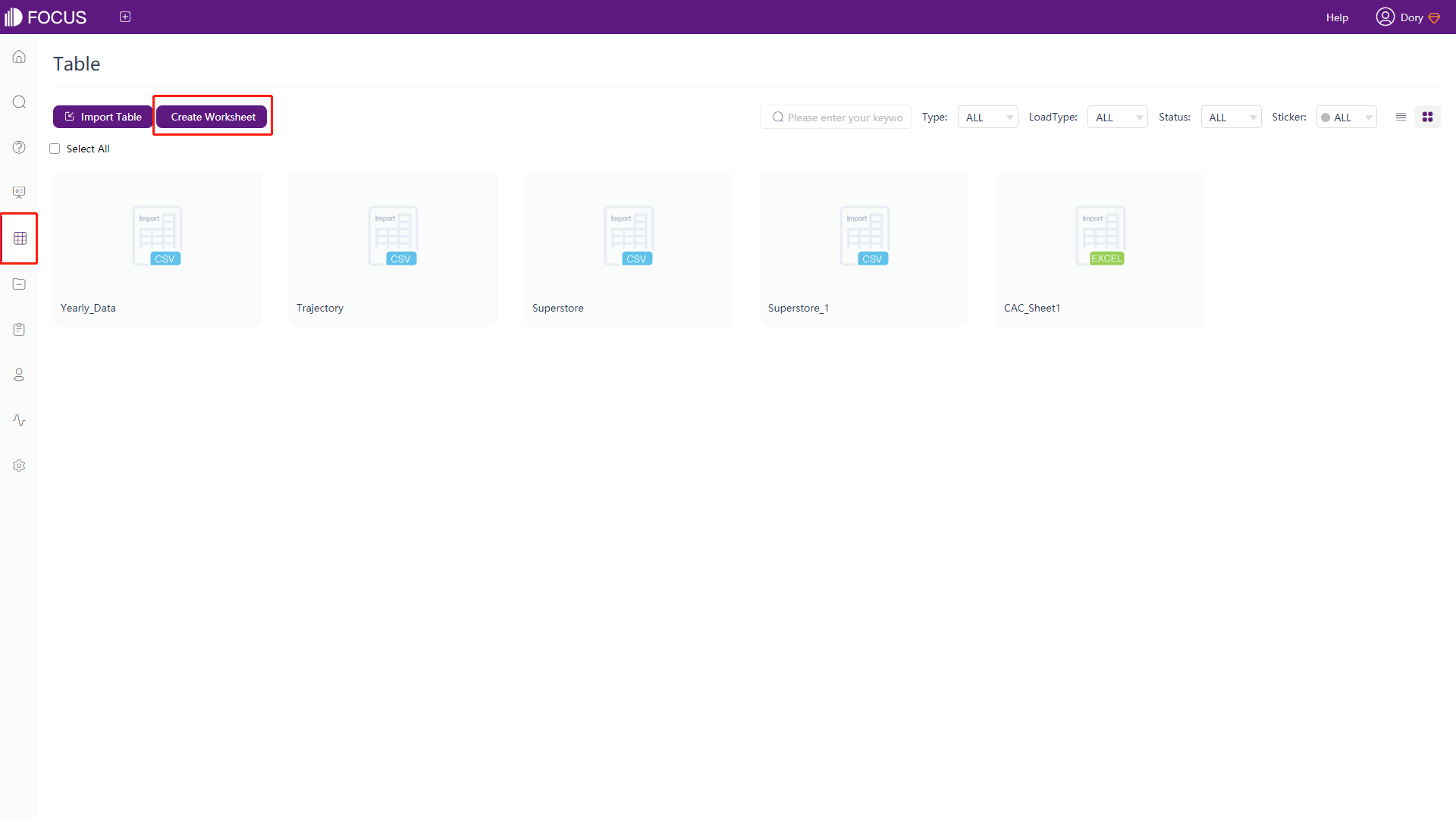
On the new page, the rest of the operations are as follows:

1. Select the data table in the upper left corner of the page, that is, select the table to be used as the data source, and the selected table will be displayed under “Choose Tables”;

2. Double-click the data column on the left or click the selected column (multiple columns can be selected), Then click the arrow button to add it to the intermediate table. The selected column name will be displayed in the middle of the page, as shown in figure 6-1-2;

3. Click “Worksheet Name” to name the intermediate table;

4. Click “Description” to describe the intermediate table (not required);

5. Click “Add formula” to add a formula in the intermediate table (the formula operation is the same as the search analysis page, not required);

6. You can click the column name under “Source Column” to directly modify the displayed column name. To modify the formula name, you need to add the formula at the bottom left, click “Formula Name” to modify (not required);

7. For the column name you don’t want to use, click the delete button directly under “Actions” to remove the column. To delete the formula, click the delete button to the right of the formula name at the bottom left;

8. If you use 2 or more data tables to create an intermediate table, you need to build the relationship between all of the selected tables in “My Relationship”. If there is already a relationship, Then clicking “My Relationship” will directly display the previously established relationship of the selected table. To create an intermediate table using multiple tables, a relationship must be established between the tables.

9. Click the “Submit” button to create the intermediate table.

   

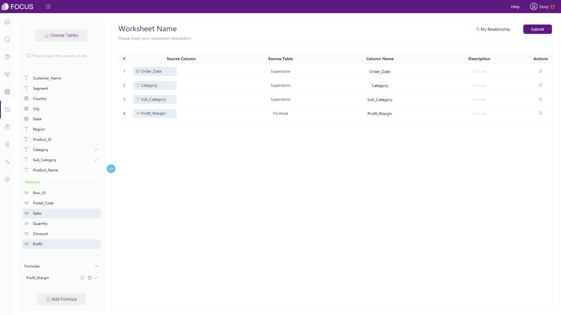
   Figure 6-1-2 Create intermediate join table

10. After the intermediate table is created successfully, you will return to the data table management module. As shown in figure 6-1-3, the intermediate tables created in different ways will be displayed as “Join-Worksheet/Question-Worksheet”, here is the setting of the intermediate join table.

    

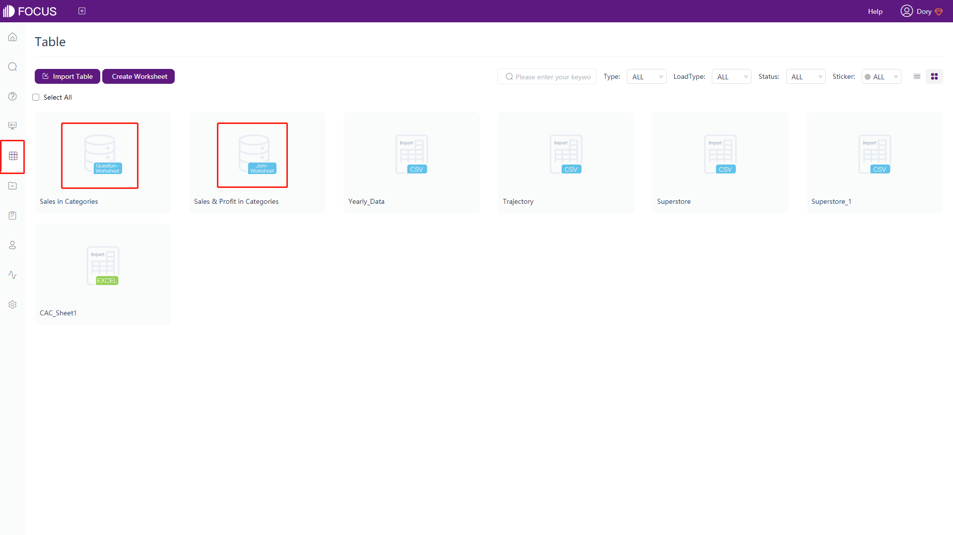
    Figure 6-1-3 Create intermediate table

6.1.2 Import Table from Local

Only users with role permissions of resource administrator can see the “Import table from locale” button under the “Import Table” column of the data table management module. Csv, excel, and json files can be imported from local. Here is an example of importing csv data:

1. Click the “Import Table” button in the data table management module, select “Import table from locale”, and the interface as shown in figure 6-1-4 will pop up;

   

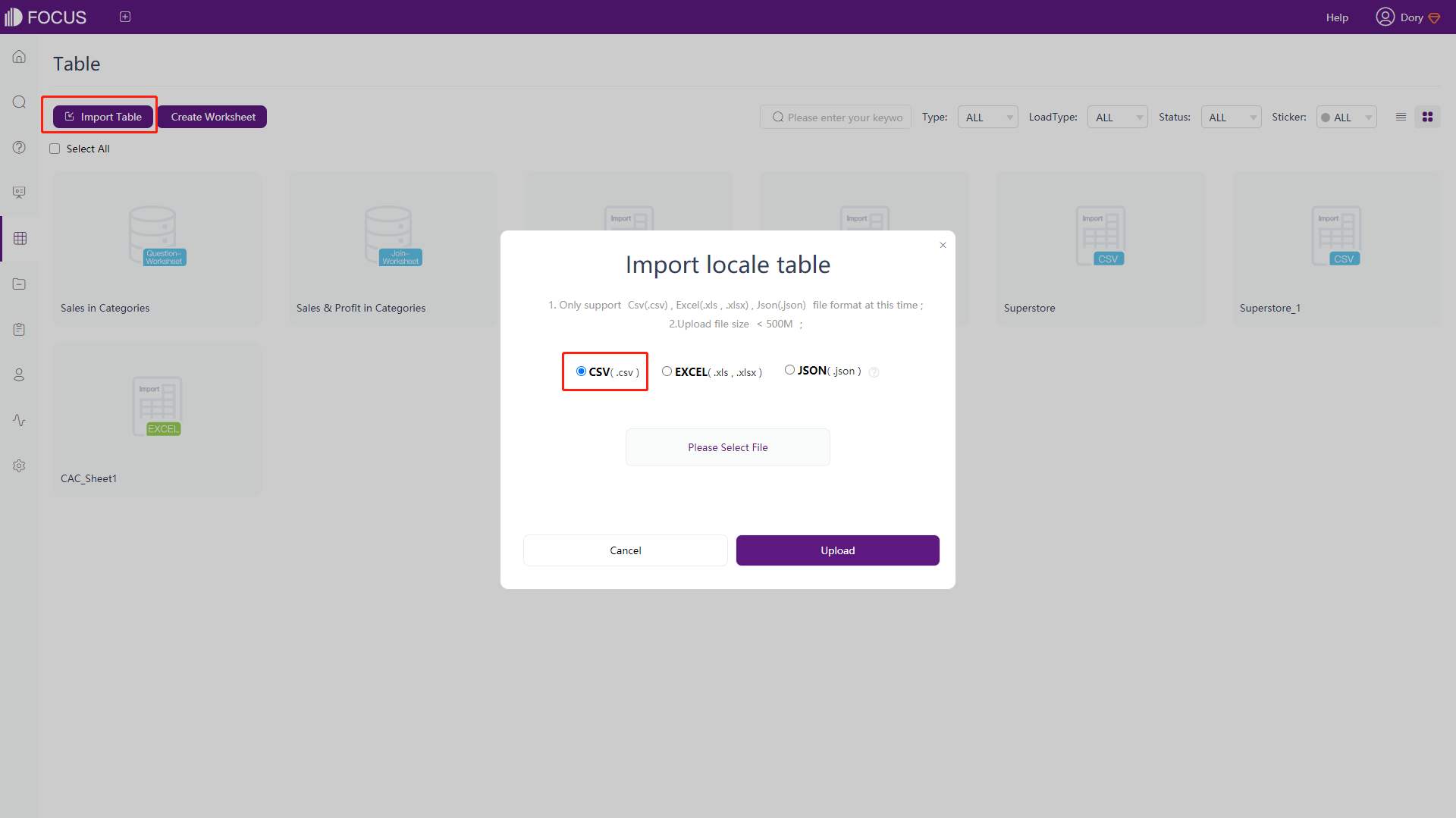
   Figure 6-1-4 Import locale table

2. The currently supported file types and file sizes will be prompted above the “Please Select File” button. Select “csv”, click the “Please select a file” button, and select the data that meet the requirements. Then click the “Upload”;

3. After the file is uploaded successfully, the configuration interface as shown in figure 6-1-5 will be displayed (csv file here). You need to pay attention to selecting the corresponding encoding rules, to correctly display the text in the imported file. Then click the “Next” after setting;

   

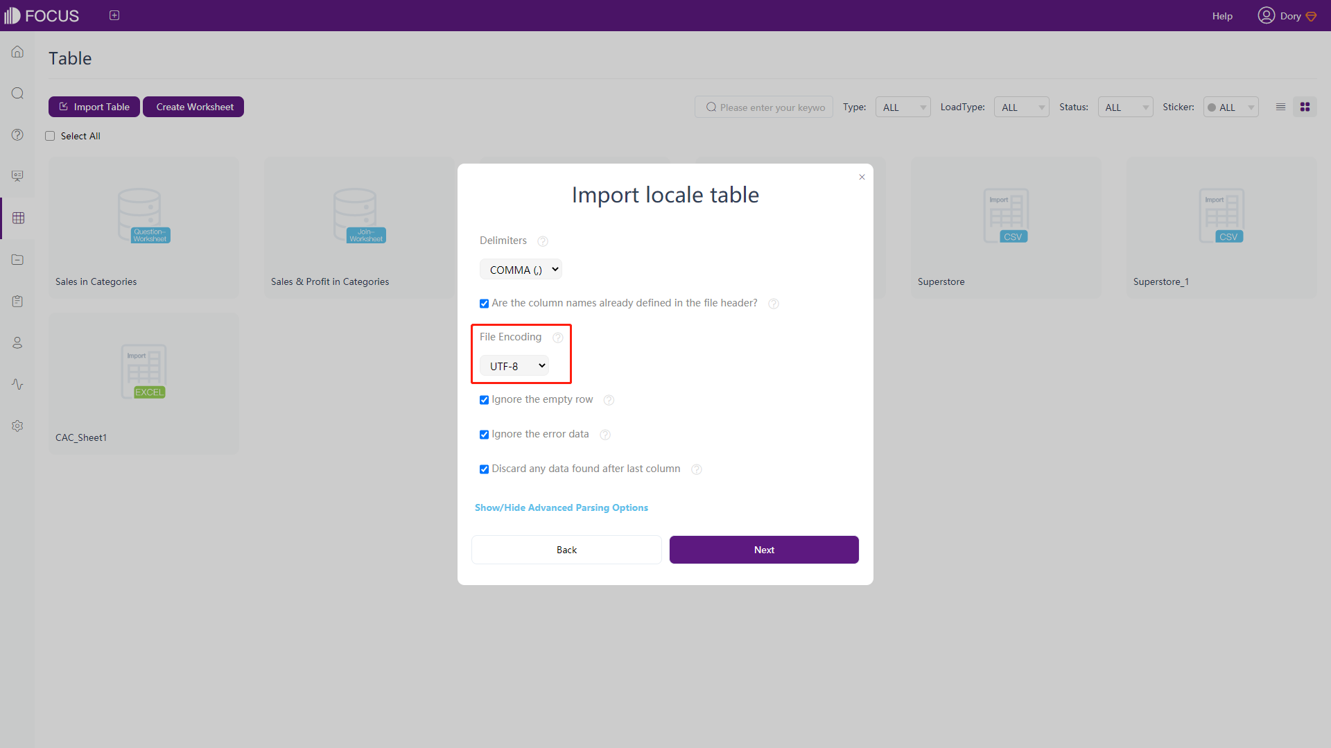
   Figure 6-1-5 Set formats & encoding rules

4. As shown in figure 6-1-6 below, you can select the column, rename the table and column, modify the column type, and preview the imported data table. After the configuration is completed, click “Submit”, the imported files will be distinguished according to the file type. For example, when importing a CSV file, CSV will be displayed.

   

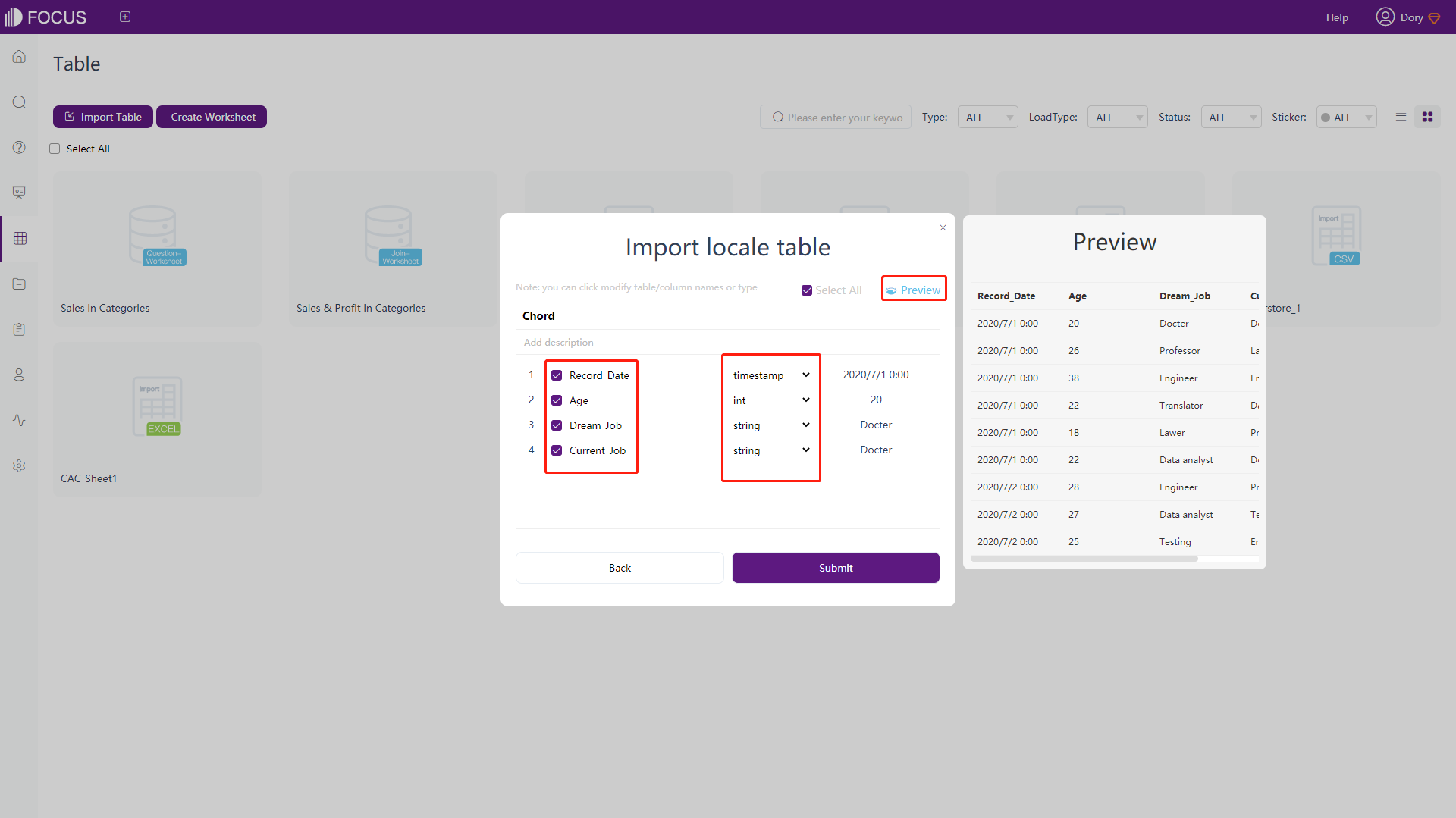
   Figure 6-1-6 Configure table columns

5. If you choose to import EXECL (.xls, .xlsx) files, you can choose to import multiple sheets. Click different sheet names, and the specific information of column Attribute will appear in the middle page. You can choose to add different columns and change the field Attributes.

6.1.3 Import from External Data Source

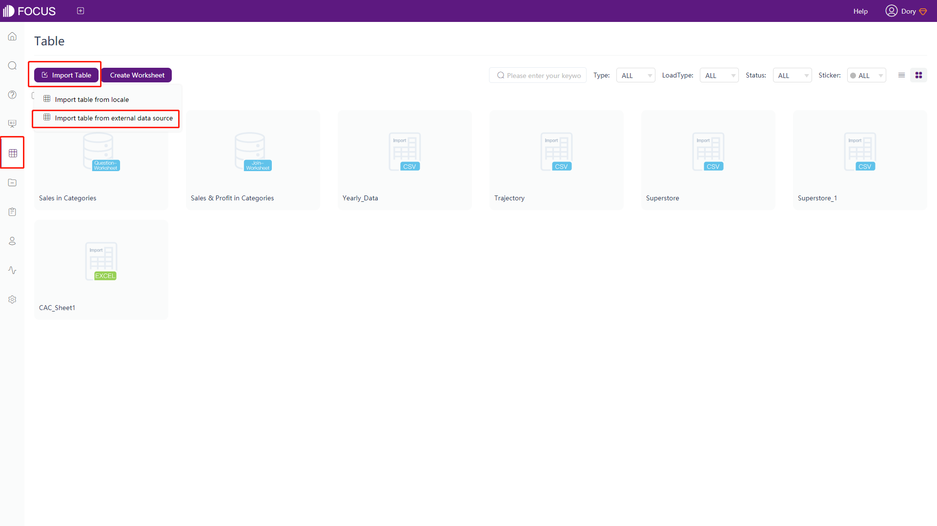
“Import table from external data source” is displayed only when users with role permissions of resource administrator. Click “Import Table” in the data table management module. Click “Import table from external data source”, as shown in figure 6-1-7.

Figure 6-1-7 Import from external data source button

1. Select data source

   On the new page, click “Please select a data source” in the upper left corner, and select the data source to be imported from the external data sources that are connected to DataFocus Cloud. Then click the “Next”, as shown in figure 6-1-8;

   

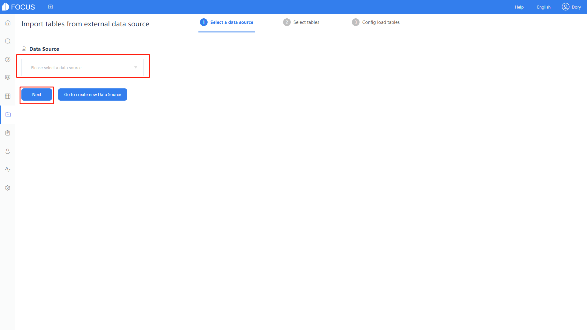
   Figure 6-1-8 Import from external data source interface

2. Select the table to be imported

   As shown in figure 6-1-9, you can select the table to be imported into the DataFocus Cloud system from the data source, and choose between direct connection and importing;

   “Import” is to use DataFocus Cloud as a data warehouse, which can integrate data in different business systems, show the full picture of the data, comprehensively analyze, and support regular refresh of imported data;

   “Direct connection” means that DataFocus Cloud directly connects to the database, and the data is not imported into DataFocus Cloud. Since the database is connected, it can support real-time update. If the data from the database changes, tables directly connected in DataFocus Cloud and the reports that rely on these tables can also be updated in real time.

   If the table has been imported, it will prompt “The table has been used”.

   After selecting the data table, click the “Submit” to go to the next step;

   

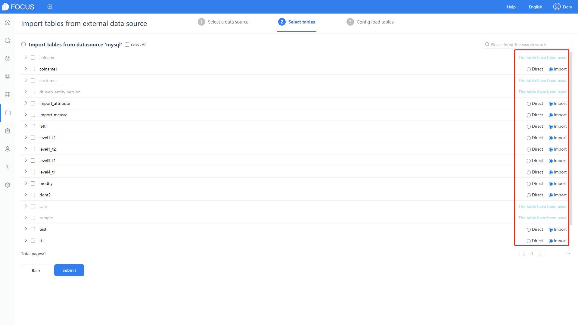
   Figure 6-1-9 Choose table from external source

3. Import Configuration

   If the import method of the selected data table is not all “Direct Connection”, that is, the import method of the existing data table is “Import”, it will go to the next step, “Configure load tables”, where you can modify the import method as full import or incremental import or direct connection, you can also configure the import time;

   There are two configurations for timing import, “Simple Repeat” and “Detailed frequency configuration”.

   Simple repeated is to input the value and select the time unit to configure the import time. For example, if you enter “every 12 hours”, the system will re-import the table according to the selected import method every 12 hours, as shown in figure 6-1-10.

   

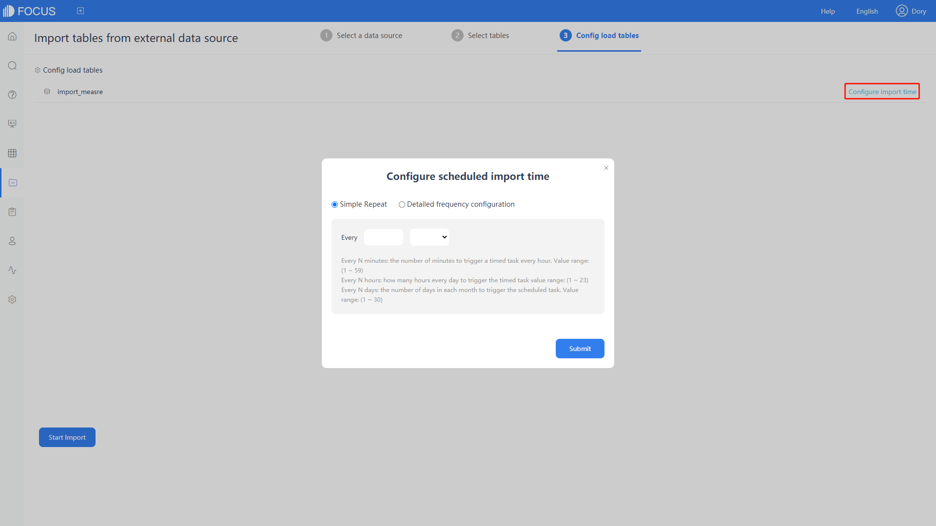
   Figure 6-1-10 Configure timing import - simple repeat

   The detailed frequency configuration can set the import time to a specific month/week/day/hour, and etc. The system will also regularly update the data source according to the set import time, as shown in figure 6-1-11.

   

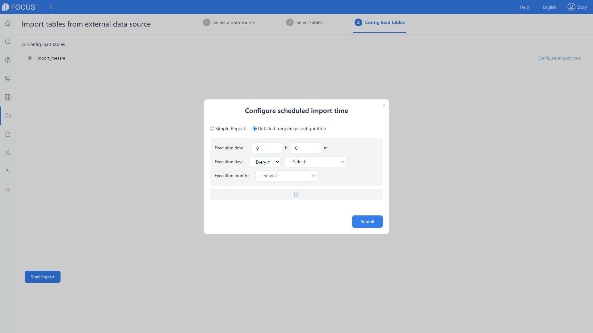
   Figure 6-1-11 Configure timing import - detailed frequency

4. Finally, click the “Submit” to start importing the data source.

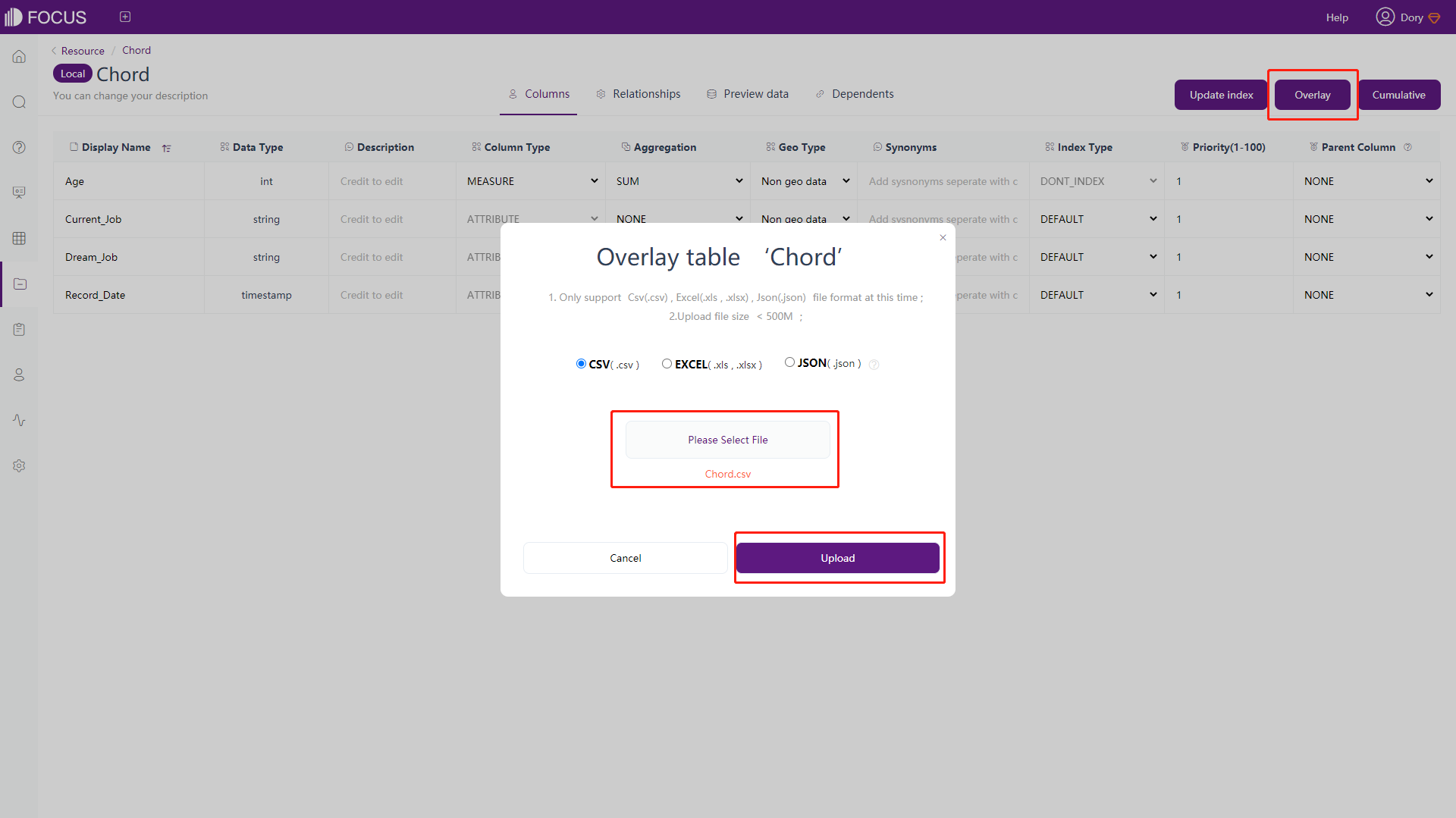
6.1.4 Override Upload Table

On table management module, click “Details” of the data table to enter the detail page. Click “Overlay” in the upper right corner, and then type in the relevant information of the data table. The steps here are the same as the steps for importing the table. After the input is completed, click the “Upload” to overwrite the original imported data table, as shown in figure 6-1-12.

Figure 6-1-12 Override table

6.1.5 Switch Data Source

When the database of original data table is changed, or when the intermediate table, answer, dashboard, etc. made of test data want to switch to use the official data, or when the data in January and the data in February need to be switched in different databases, we need to switch data sources for data replacement. When the table names and the structure is the same, by editing the specific link configuration of the data source, the imported table under the current data source can be replaced with table of other data source. After the replacement is successful, the content of the intermediate table, answer, and dashboard created by the original data source will be updated according to the new data.

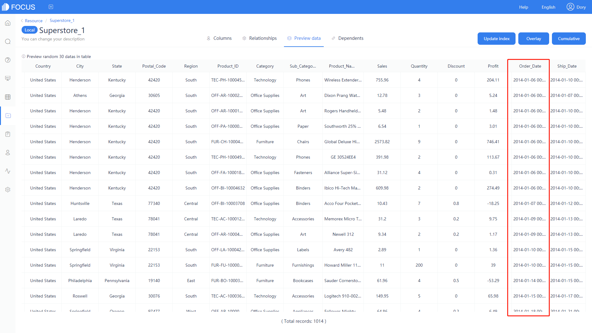
Here we take switching “Data Source 1” to “User Data Source” as an example.

We can see the detail page of the data table “Superstore” in the user data source, showing the data for 2014.

Figure 6-1-13 Data from external source

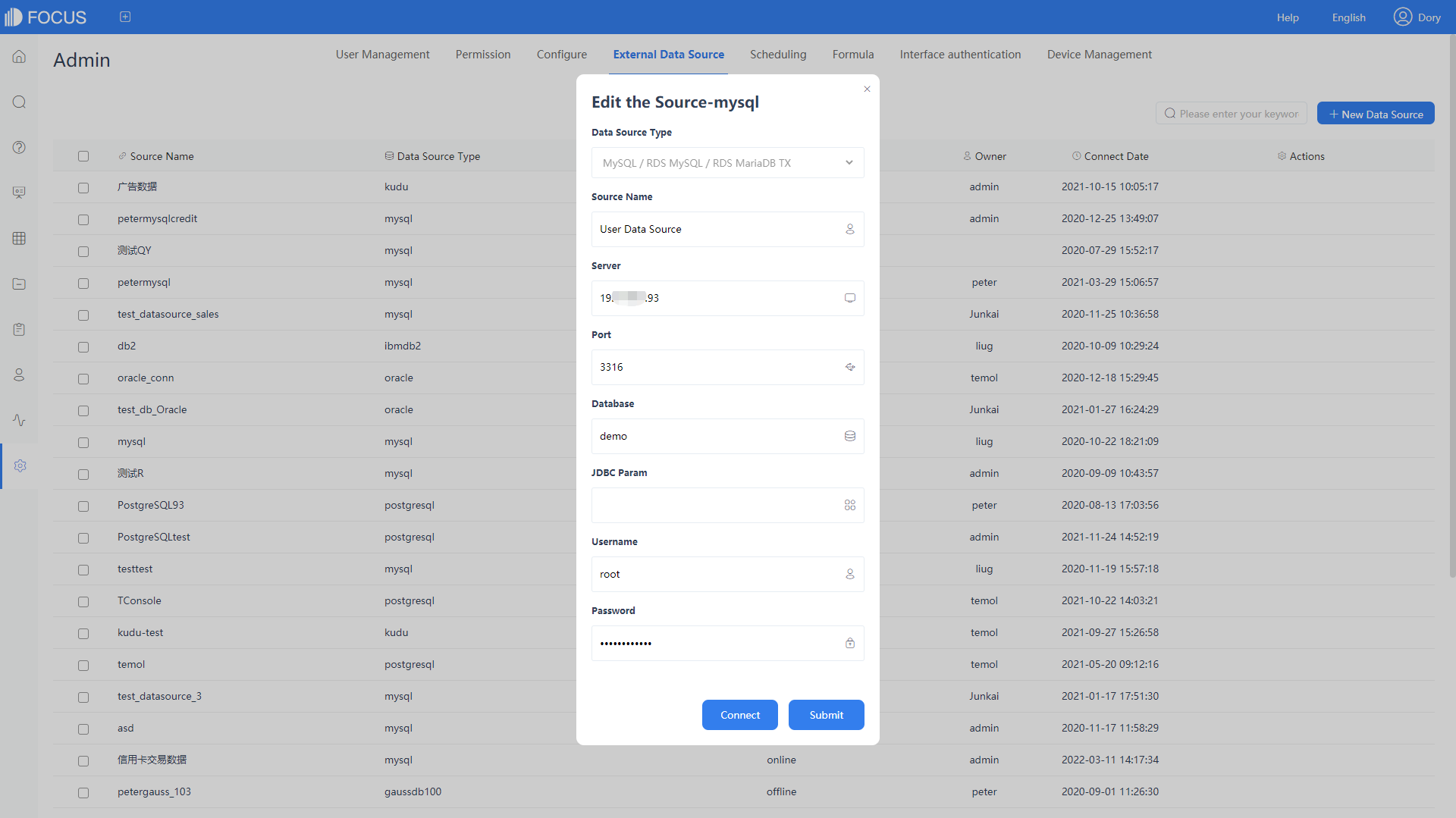
Click External Data Source in System Management, click Edit, enter the data source configuration information of Data Source 1, and click the “Submit”.

Figure 6-1-14 Switch external source

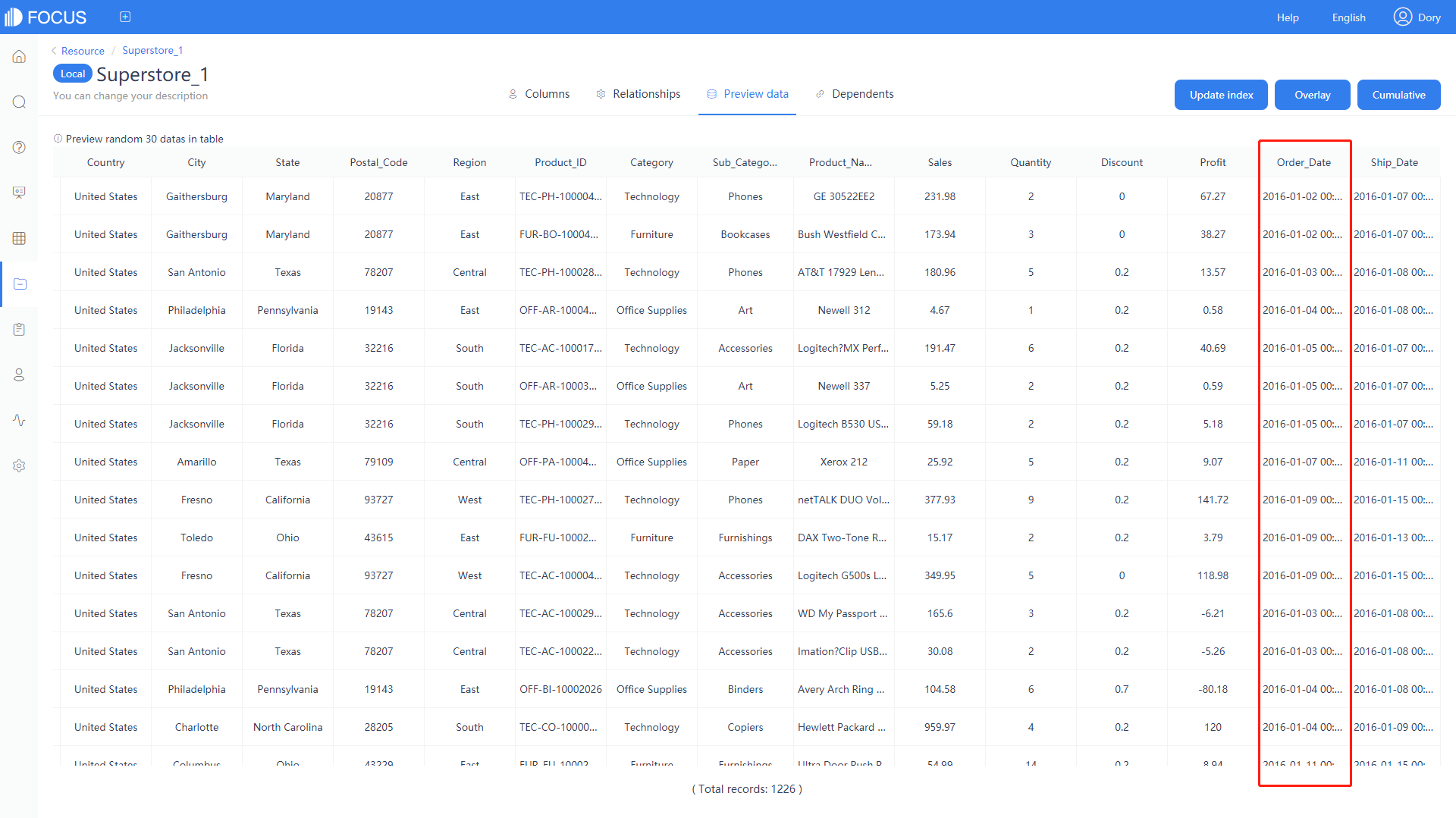
Then on the data table management module, click the “Detail” button of table “superstore”, click to preview data. The data has been replaced with the data in 2016.

Figure 6-1-15 Replaced data

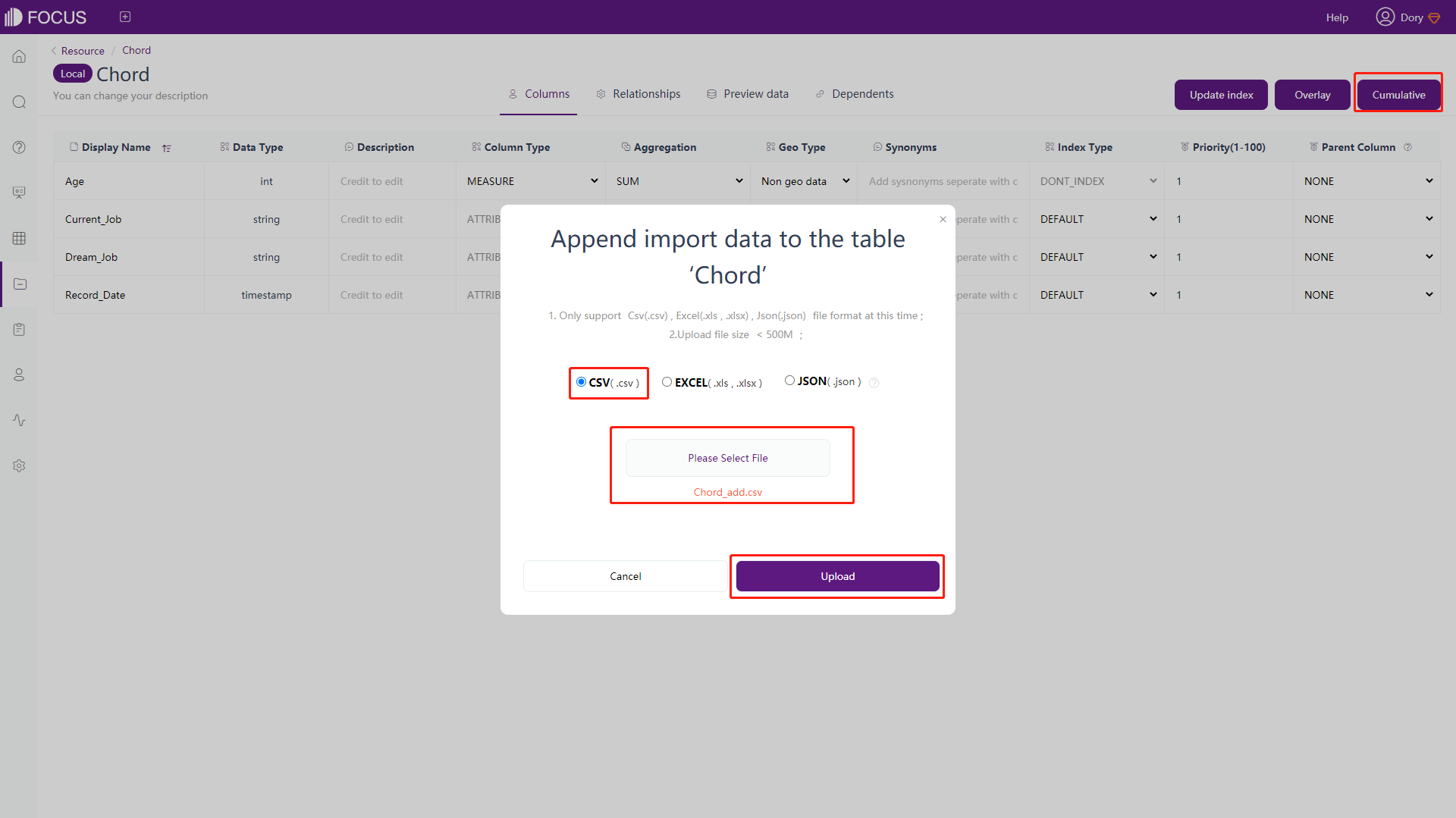
6.1.6 Cumulative Upload Table

When new batch data needs to be added to the data table, the cumulative upload function can be used to add new data to the original table. Click “Cumulative”, select the table to be added, and click the “Upload” to add data, as shown in figure 6-1-16.

Figure 6-1-16 Cumulative upload table

6.2 View Data

There are two data sources: import and direct connection. Imported data is stored in the system, which can be directly retrieved for use. Directly connected data is connected to the user database. Unlike imported data, it is not stored in the system. The query is made in the database and then results are returned to the system for display.

There are three types of data: data table, intermediate answer table, intermediate join table.

The intermediate table is obtained after secondary processing of the source data table. When the structure of the source table changes, the intermediate table will be affected; intermediate answer table is generated on the search analysis page, intermediate join table is generated on the resource management module. The difference between the two is that the answer intermediate table will perform data aggregation when it is generated, while the intermediate join table will not.

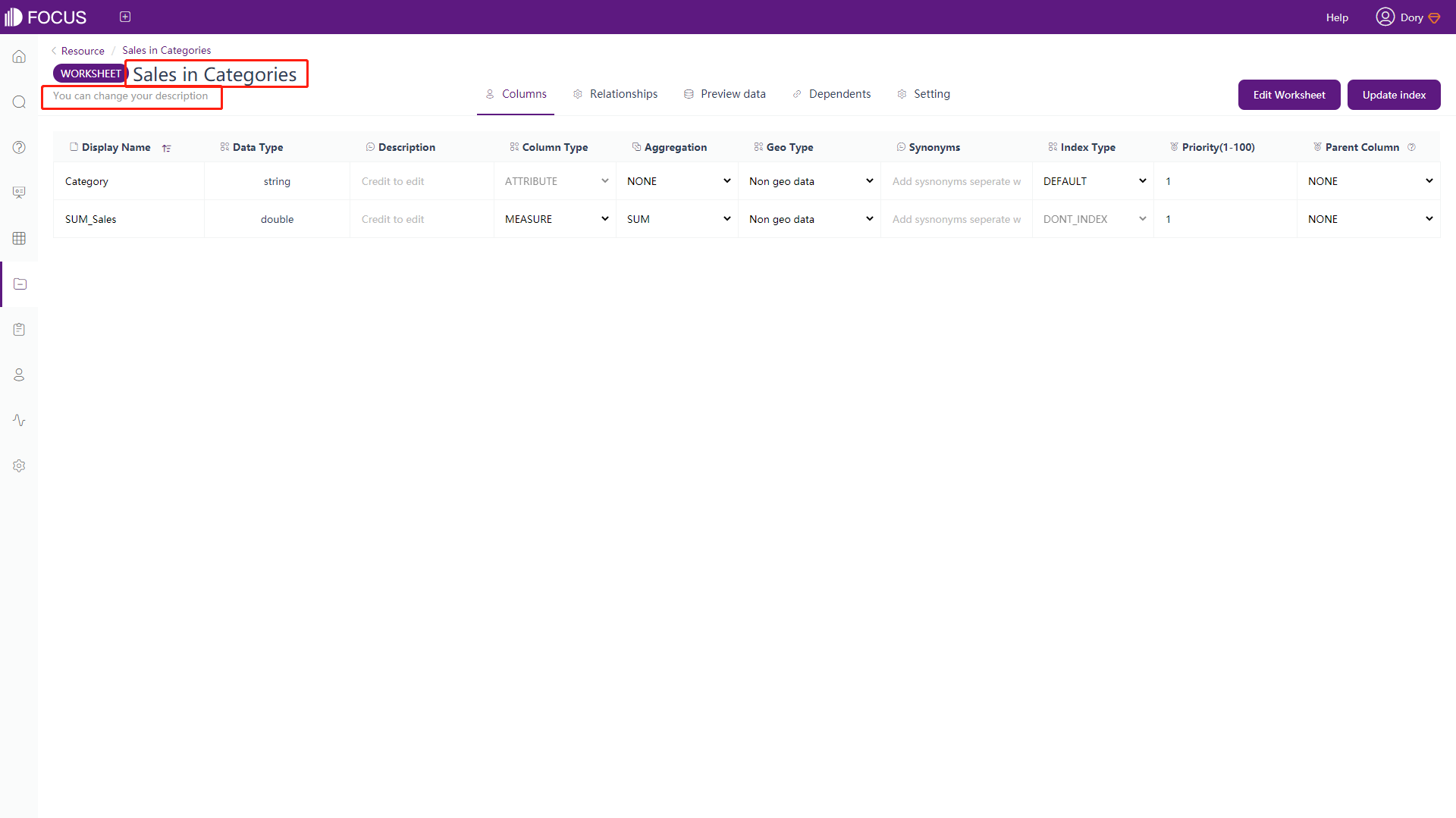
In the table management module, click on any table (Click the “Detail” for thumbnail layout) and the interface shown in figure 6-2-1 will pop up. Click the title name and description in the upper left corner can be directly modified.

Figure 6-2-1 Detail page of table

6.3 Data Content

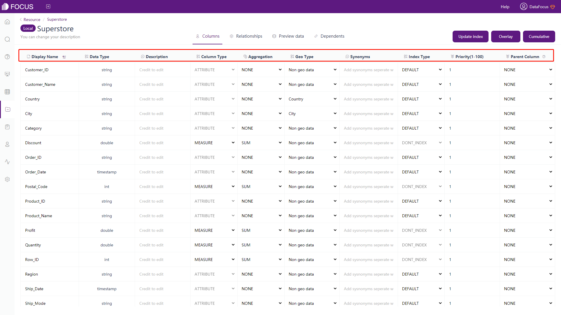
6.3.1 Column Information

In the column information, you can see the information of each column in the table, such as displayed name, data type, description, column type, aggregation method, geographic type, synonym, index type, priority and parent column, as shown in figure 6-3-1.

● Display name: The displayed name of each column.

● Data type: The data type of the column is fixed during the import and cannot be modified here.

● Description: The description of the column field, users can add according to own needs.

● Column type: There are two types of columns: Attribute and Measure. The Attribute column is generally used as the X-axis and legend, and the Measure column is used as the Y-axis. Measure columns can be modified for use as Attribute columns.

● Aggregation: The aggregation method of each column. The numeric column has 8 aggregation methods: sum, maximum value, minimum value, average value, variance, standard deviation, count, and deduplication count. Generally, the default is the sum, or you can choose not to perform aggregation. The Attribute column has 2 aggregation methods: count and deduplication count. Generally, the default is no aggregation. Users can make changes in the column information, and can also use settings and keywords to make temporary changes in the search.

● Geo type: Configure the geographic column, and configure the corresponding column as state, city, district, and longitude and latitude. The column is required to conform to the format and value of a geographic column.

● Synonyms: the synonym name of the column, which can be used as a substitute for the displayed name in the search, and the effect is the same as the displayed name.

● Index Type: Select the modeling method.

● Priority (1-100): When a filter condition is entered in the search box, the result will have an aggregated Measure column. The results of Measure column with higher priority will be displayed first.

● Nested parent column: Select an Attribute column of the same type to form the tree index. In the “Nested parent column” column of the child column, select the parent column.

Users with resource management permissions can modify the content in the column information of the data table. An error message will appear when the modified column name and its synonym are duplicated with the keyword.

After modifying the information, reopen it to see that the information has been changed. If you changed a column name in the table, you can see in the search module that the column name has been replaced with the modified column name.

Figure 6-3-1 Column information

6.3.2 Join Tables

User with the resource administrator role can join data tables.

1. Add a new join

   If you want to add a relationship between the current table and other tables, enter the relationship page from the detail page. If the table has not joined with any other table, the relationship page will only display two buttons: “Add Relationship” and “View all Relationship”.

   Click “Add Relationship” at the top left, and the interface will pop up as shown in figure 6-3-2. You need to fill in the information includes dimension table, join type, join filter (optional), source column, and destination column.

   

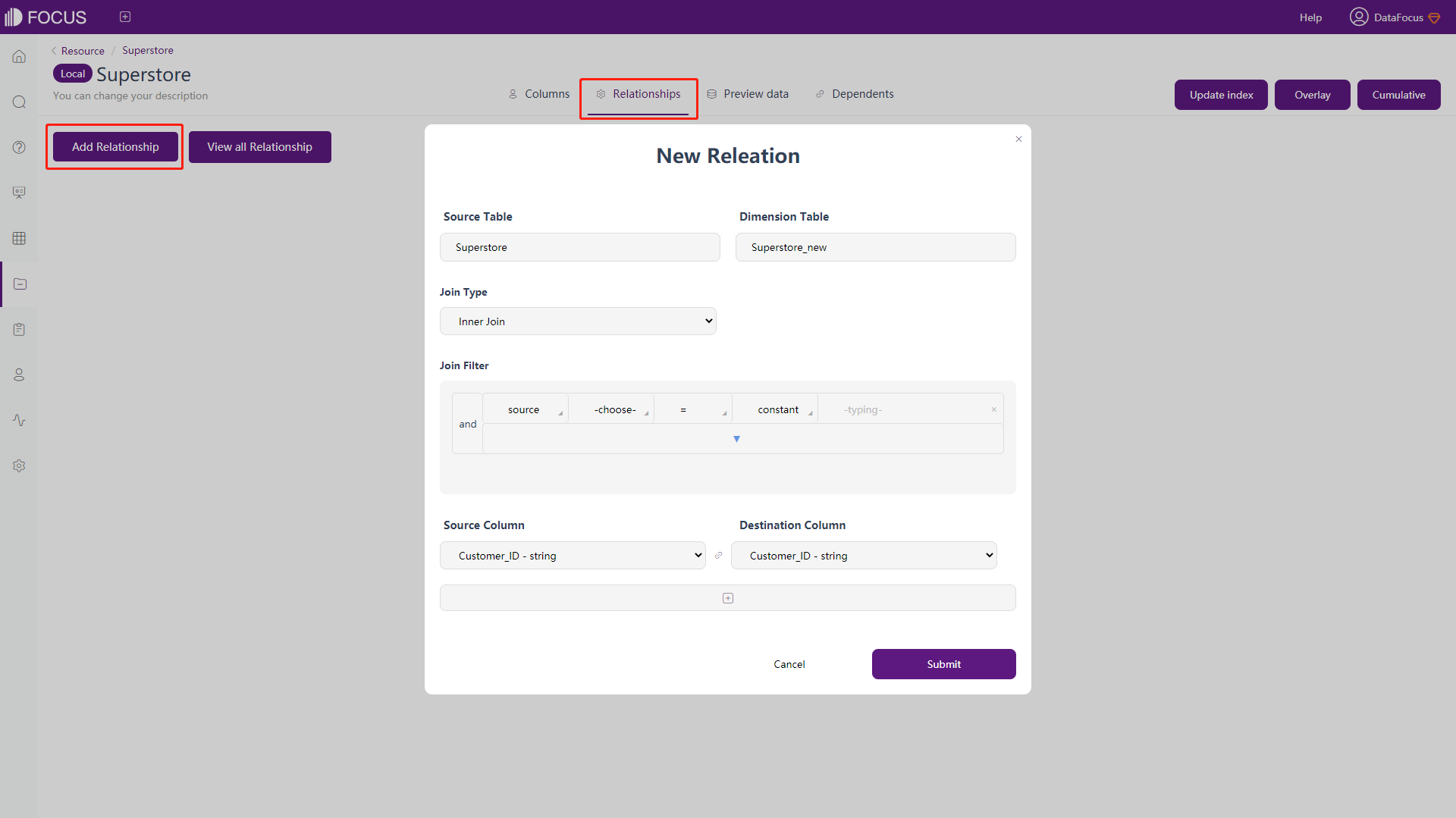
   Figure 6-3-2 Add relationship

   Dimension table refers to the data table to be associated with the current table. Click the input box of the dimension table, and the top 10 tables in the system will appear. If the dimension table you want to join is not among them, you can enter the name in the search box, and then select the table you want to join;

   There are four types of joins: inner join, left join, right join, and full join;

   Join filtering is to filter related rows of data, and select the Attribute column or Measure column of the original or target column to establish filtering conditions;

   The source column is to display all the columns in the current table. Clicking the input box will display all the column names and their data types;

   The target column is to display all the columns in the dimension table. Clicking the input box will display all the column names and their data types;

   After selecting the data column to be matched, click “Submit” to add the relationship. If there are multiple columns that need to be related to a dimension table, you can click the “+” button below the source column to add input boxes for new source columns and target columns.

   When creating a relationship, the join cannot have loops or closed loops.

2. Association details

   After the relationship is created, move the mouse to the connection line between the two tables, and the “Detail” button of the relationship will be activated, as shown in figure 6-3-3. Click “Detail” to view the details of the current relationship, including dimension tables, connection types, Connection filter (optional), source column and target column, as shown in figure 6-3-4.

   

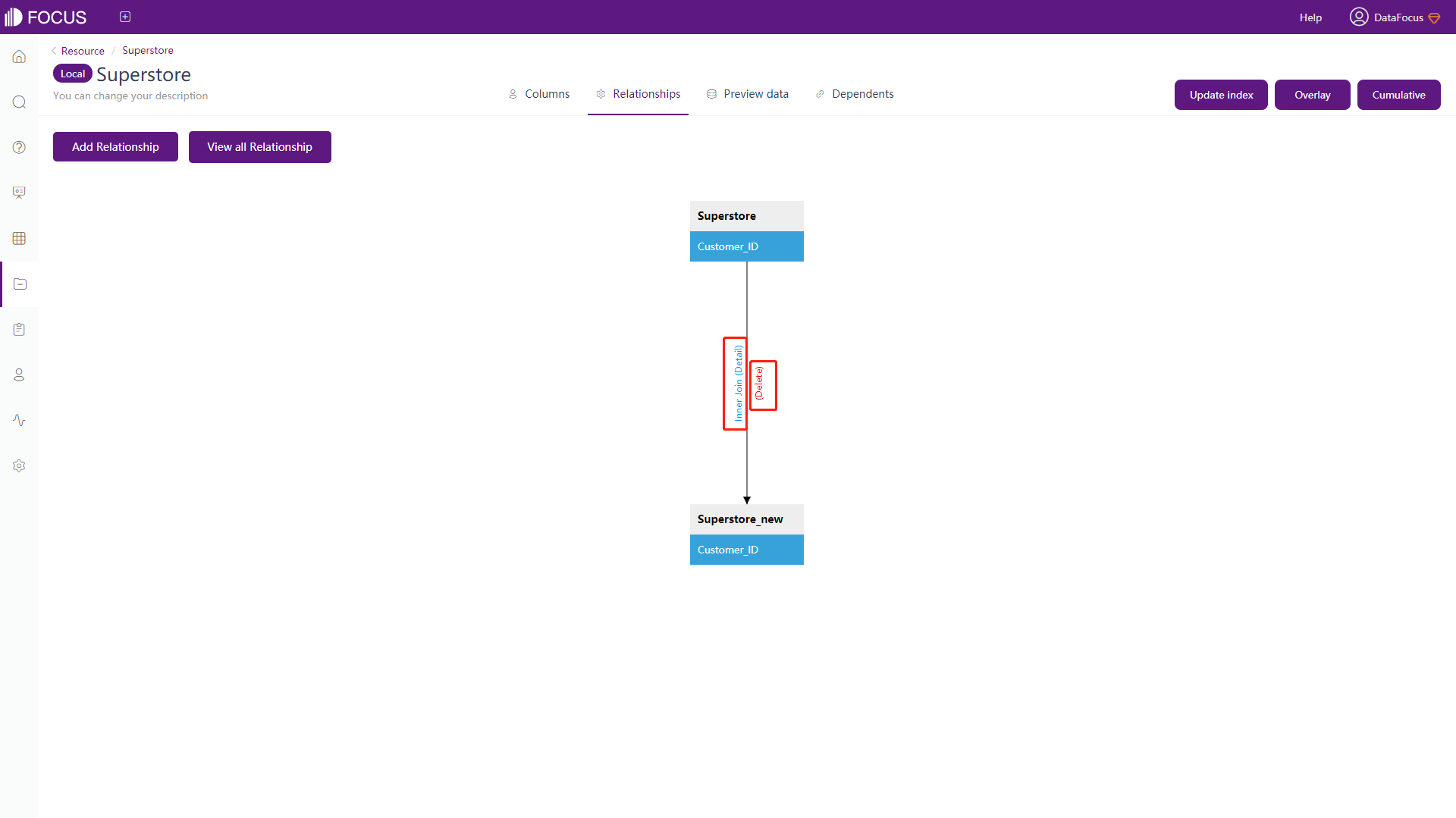
   Figure 6-3-3 Relationship detail button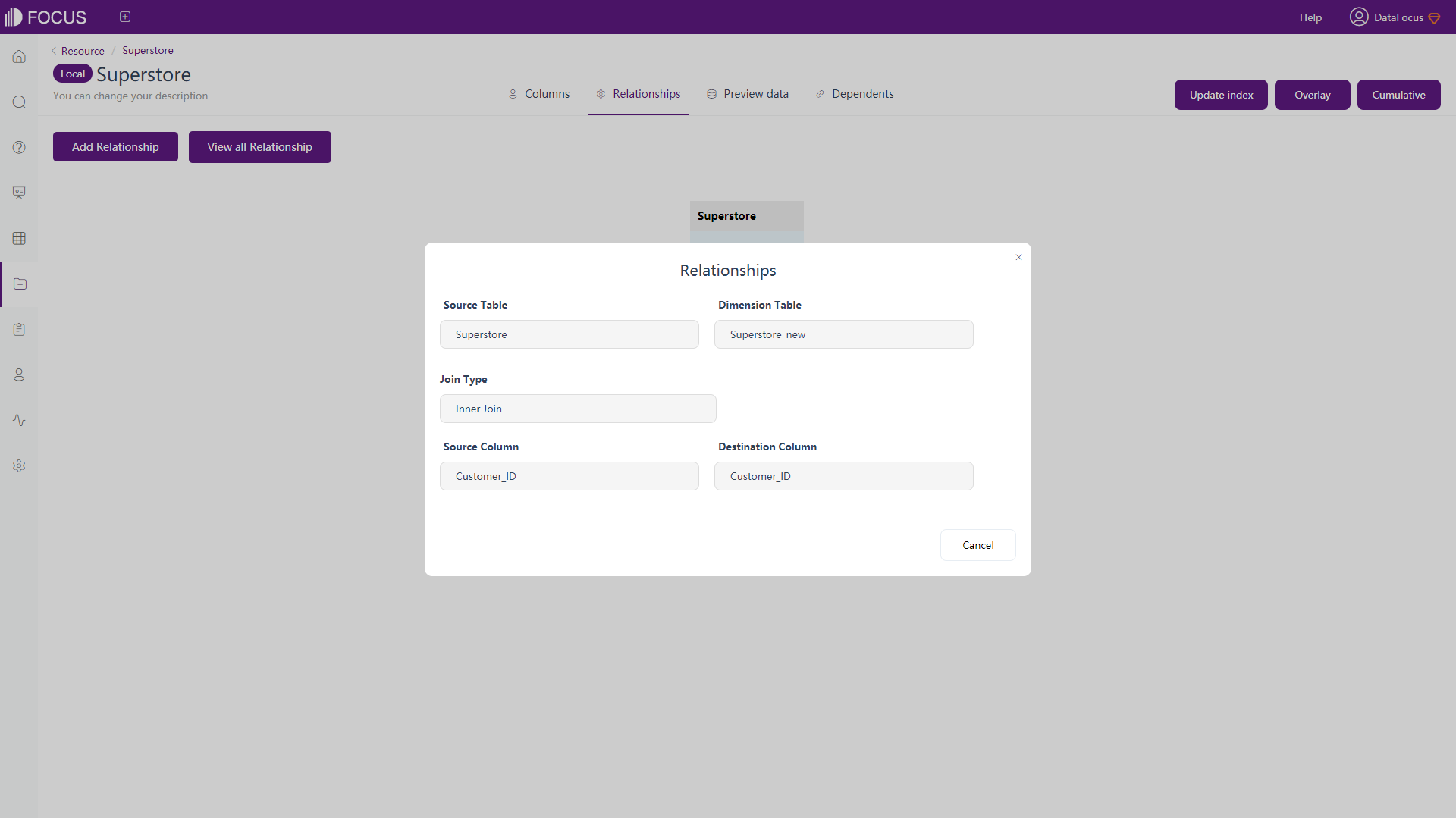

   

   Figure 6-3-4 Relationship detail page

3. Delete relationship

   If you want to delete the relationship between the two tables, move the mouse to the connection line between the two tables, the “Delete” button will be activated, as shown in figure 6-3-3. Click the “Delete” to remove the relationship between the two tables, as shown in figure 6-3-5 below.

   

   Figure 6-3-5 Delete relationship

4. View all relationships

   When you want to view the relationship of all tables macroscopically, or are unclear about the relationship between the tables due to time or other reasons, click “View all Relationships” in the upper left corner of the relationship page, as shown in figure 6-3-6. Enter the overview page of the join relationship of all tables, as shown in figure 6-3-7.

   

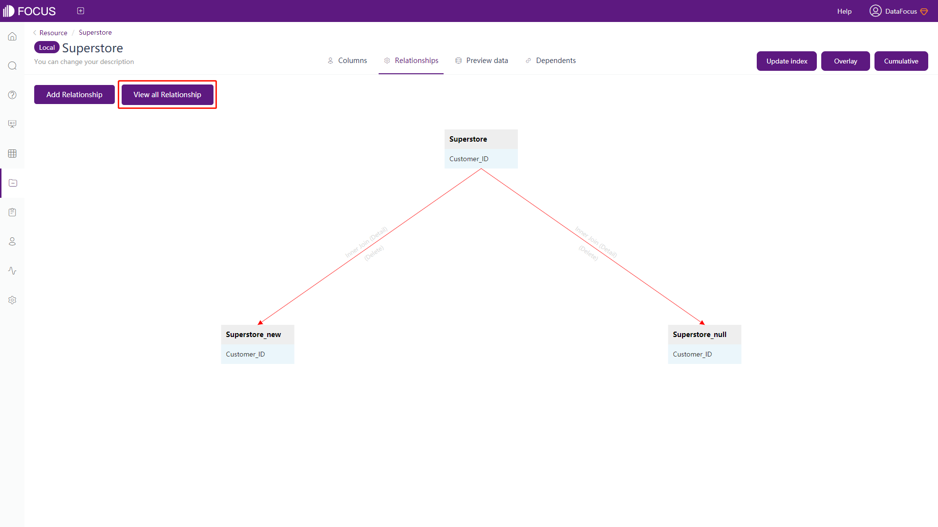
   Figure 6-3-6 View all relationships button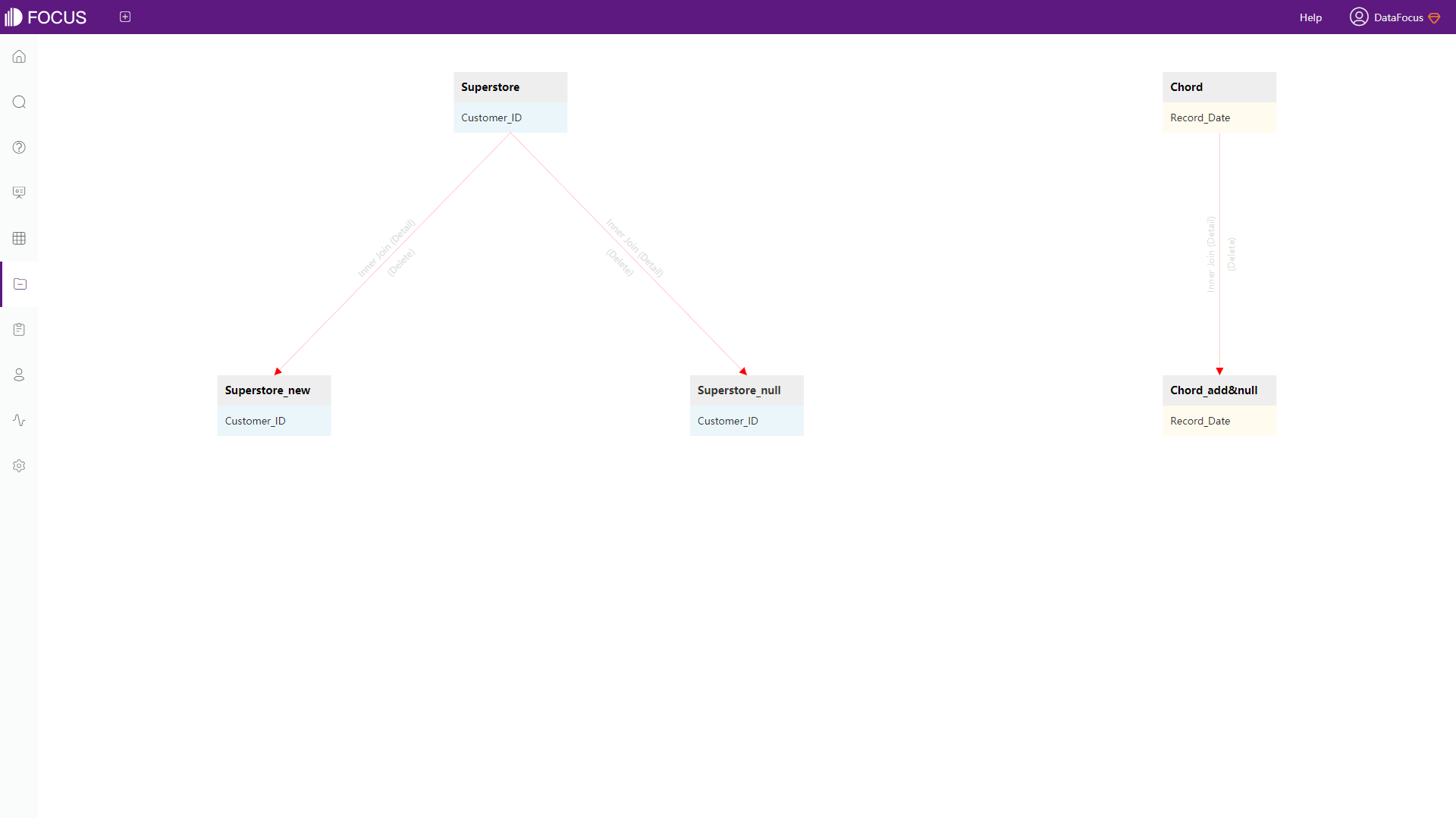

   

   Figure 6-3-7 View all relationships

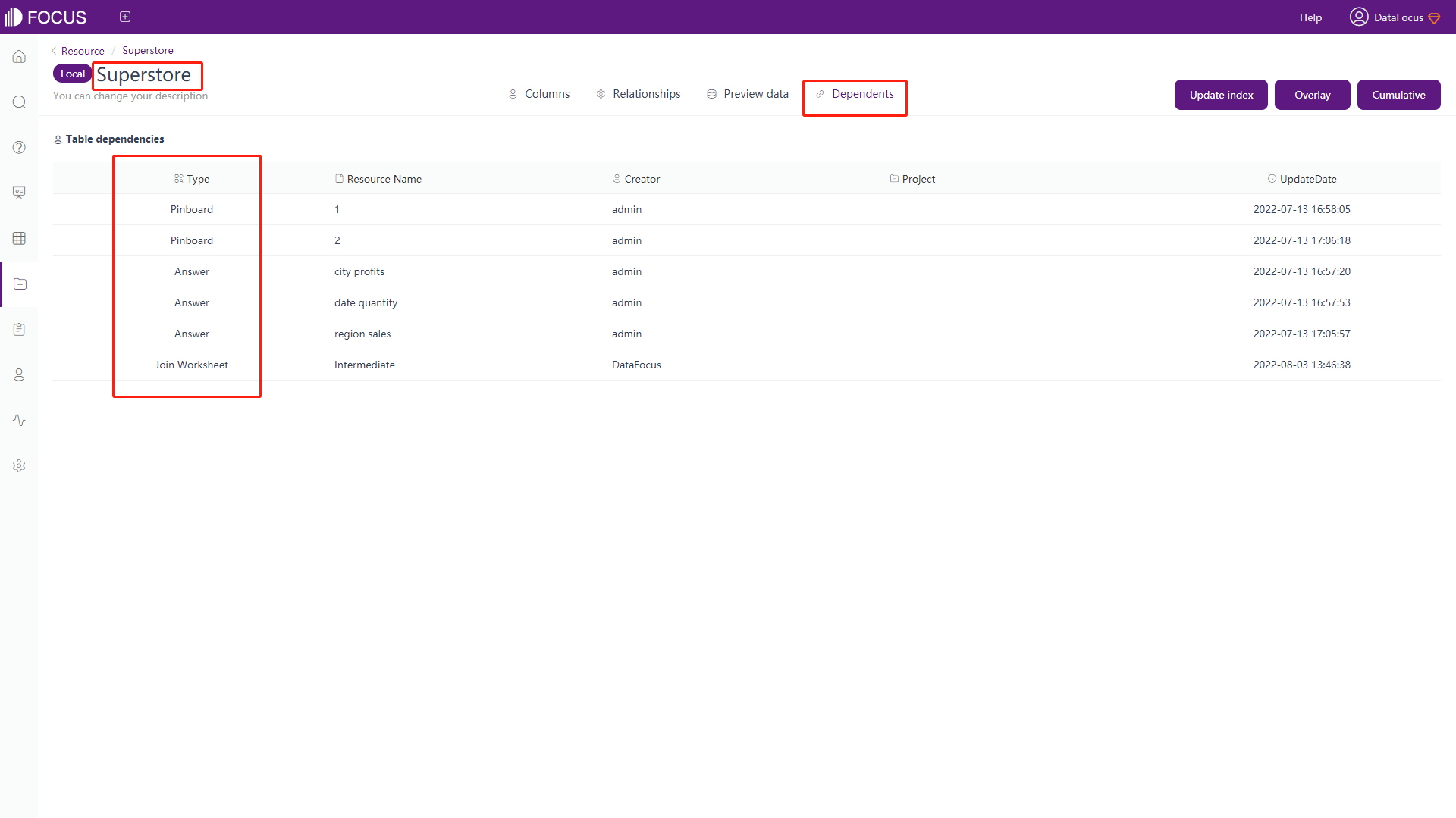
6.3.3 Dependence

Click the “Dependents” on the detail page, and you can see the dashboard, answer and intermediate table built on the current table, as shown in figure 6-3-8 below.

Figure 6-3-8 Dependents